pyXsurf - a Python library for analysis of surface data
Outline
- Surface Metrology and AFM
- What is pyXsurf, and why you need it
- Some examples
Surface Metrology Data for AFM and Other Instruments
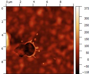 | 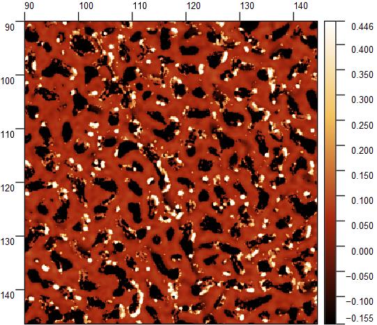 | 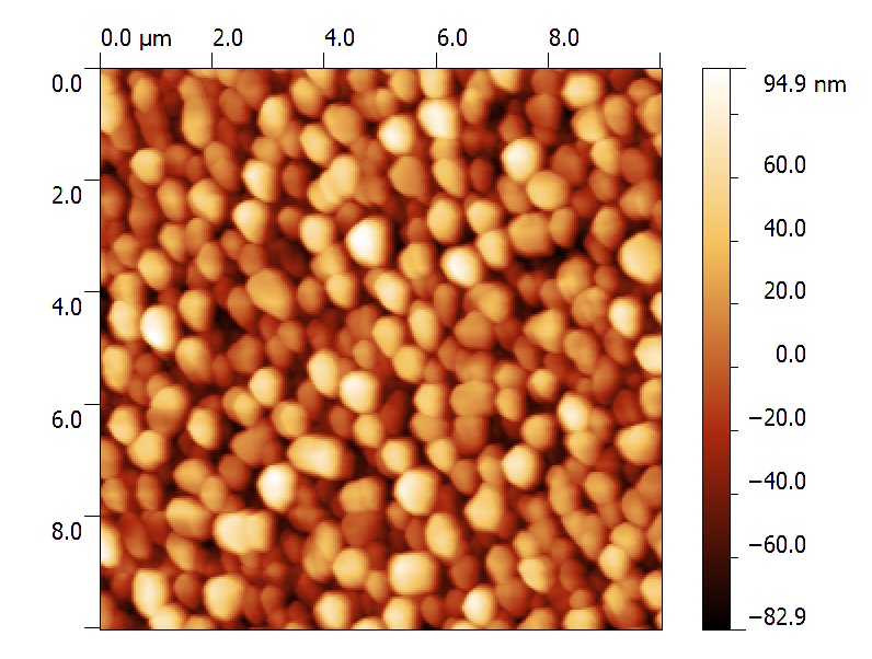 | 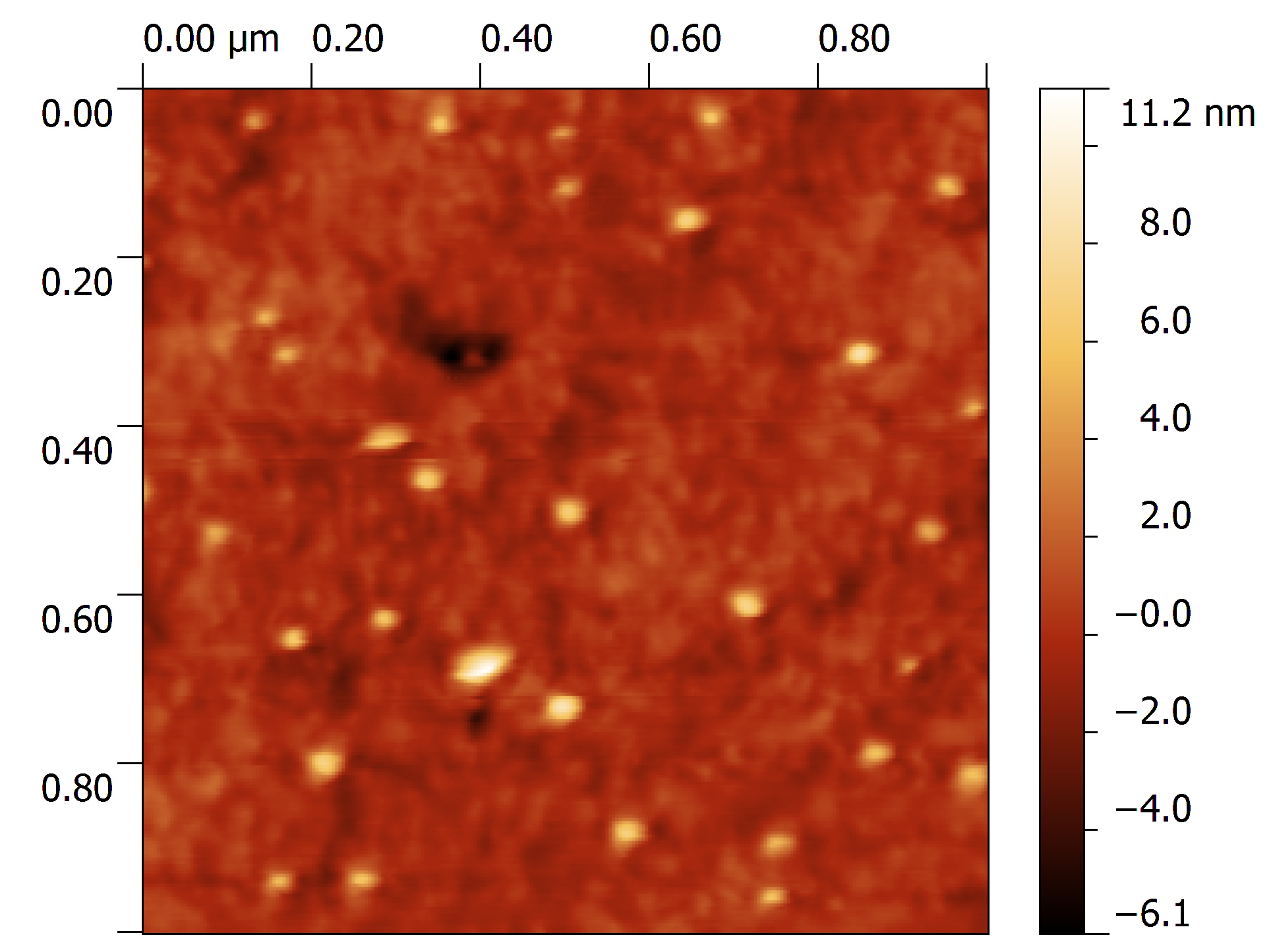 |
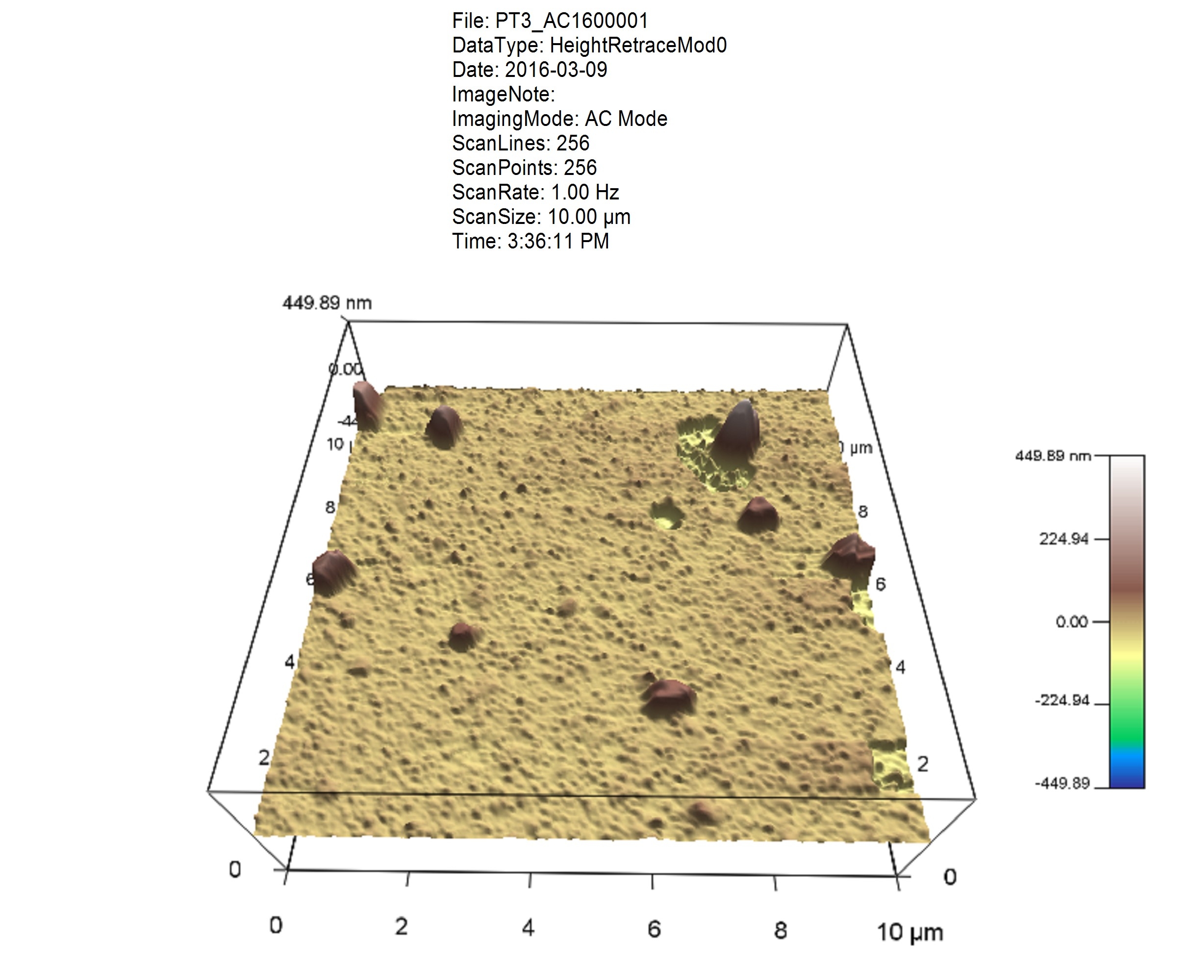
AFM data are (most of the times) surface or profile data.
Surface and Profile data (I will consider them as a subset) are of general interest in almost any field of science and technology, from optics, to microscopy, to material science and biology.
Many operations are common to different disciplines and instruments.
Data represent a map over a 2D grid (or more in general a set of points in the 3D space), where elevation, intensity, or other quantities are expressed as a function of 2D position, identified on surface by its relation with coordinate axis.
A set of operations (many of which are common in different disciplines, e.g. leveling, feature recognition, profile extraction) are performed on data.
Furthermore:
- Automatic metrology systems can collect large sets of correlated data.
- Several related maps (e.g. different instruments or different samplings) can be correlated.
- There might be automation/interaction with other instruments or sensors.
Common Solutions and Tools
OEM Software
Usually provided with the instrument. Typically GUI-based:
- quick and easy, however can be a problem for consistency (e.g. change of color scale, different leveling procedures).
- It needs a skilled technician to manage settings, analysis and macros. Hard-to-acquire and instrument-specific skills.
- limited or no access to code to add functionalities (*)
- not scalable to large number of data (*)
(*) Many of these tools implement some form of scripting (often Python based) or macro procedures, internally (scripting engine embedded in software) or externally (access to internal functions given through APIs od DLLs).

|  |
 |
Open Source Solutions
|
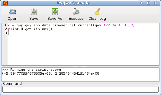
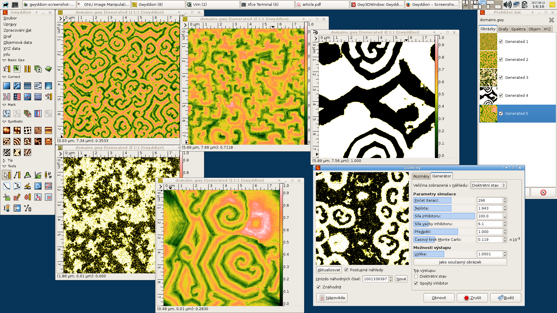
Gwyddion, developed for nanometrology, and probably the most successful software of this kind, is versatile and can handle many formats of surface data. It offers open source and has some form of interfacing with python, but is still based on a very proprietary graphical interface. |
 |
In Academy
 |
Everybody writes their own software:
|
The Python programming language impact on science
In many fields of science, the Python programming language, with its approach aimed at reusability, inverted this tendency: in the last years, several Python packages, tools and libraries emerged and established themselves as standard tools, bringing the language to be one of the most popular in science, if not the most popular.
 |  |
The result is an enormous base of users.
High quality libraries for practically any field of science.
Python is likely also the most commonly used language for scripting of surface-metrology instruments proprietary software.

However, to the knowledge of the author, there is not an universally recognized framework in any language and especially not in Python.
Python has good facility to deal with multidimensional arrays, but it lack the coordination with axis (It basically treat everything as a matrix).
pyXsurf
The library was created during research on X-ray mirrors (X-ray mirrors are characterized at all wavelength from AFM to LTP, meaning from 1 um to meters scan size, profile or surface).
The pyXsurf library consists in a set of core routines and classes, with a quite uniform and well defined interface, which can internally handle coordinate transformations, resulting in much more intuitive operations and enabling complex actions on data compared to pure Python.
Advantages of the approach
Python offers:
- Numerous facilities and tools available for software maintenance and documentation: tests, API documentation;
- Solid development environments, debugging tools, package managers;
- Reusable code;
- Different interfaces (command line, scripts, notebooks, graphical interface or integration with existing code, interactive code to share online), making it the ideal language for an easily-maintainable general-purpose project.
- Huge amount of high-quality science libraries;
- Highly reusable code;
Structure of the library
The library is mostly made of classes, of which the most important is Data2D, representing a measured surface. A Data2D object p1 can be created by passing data, e.g.:
from pySurf.data2D_class import Data2D

D = Data2D(data,x,y,units=['um','um','nm'],scale=[1,1,1.e9],name=os.path.basename(f))  # data,x,y previously read from .dat file
We can do a basic plot.
D.plot(stats=1)
<Axes: title={'center': 'M12 no corona 50 nc.dat'}, xlabel='X (um)', ylabel='Y (um)'>

The units are already set up. Several options are available for customization, plot method follows standard plt.plot interface, the returned plot is an plt.Axes object, modifiable with usual commands.
Leveling can be performed with a number of options to level to same or different orders in x and y, or by line along each axis:
D.level?
Signature: D.level(*args, **kwargs)
Docstring:
level_data(data, x=None, y=None, degree=1, axis=None, byline=False, fit=False, *args, **kwargs)
Use RA routines to remove degree 2D legendres or levellegendre if leveling by line.

    Degree can be scalar (it is duplicated) or 2-dim vector. must be scalar if leveling by line. Note the important difference between e.g. ``degree = 2`` and
      ``degree = (2,2)``. The first one uses degree as total degree, it expands then to xl,yl = [0,1,0,1,2,0],[0,0,1,1,0,2]. The second

    leveling by line (controlled by axis keyword) also handle nans.
    x and y are not used, but maintained for interface consistency.
    fit=True returns fit component instead of residuals

File:      c:\users\kovor\documents\python\pyxtel\source\pysurf\data2d_class.py
Type:      method
Leveling operations return a new object, Commmands can be chained, here plot method is called on the object resulting from D.level() (default remove plane):
plt.figure(2)
D.level().plot(stats=1) # remove plan, stats controls the info box
<Axes: title={'center': 'M12 no corona 50 nc.dat'}, xlabel='X (um)', ylabel='Y (um)'>

Statistical functions (same interface as plt.hist()):
D.level().histostats(); # data after plane removal

The distribution is quite irregular, we can look for a more advanced leveling.
Results can be assigned to variables, here Dl is the result of removing a plan and then second order Legendre in horizontal direction for each line is removed:
plt.figure(3)
Dl = D.level().level(2,axis=1)
Dl.plot(stats=1)
<Axes: title={'center': 'M12 no corona 50 nc.dat'}, xlabel='X (um)', ylabel='Y (um)'>

Several common operations, remove outliers:
plt.figure()
Dl.remove_outliers(nsigma =3).plot()
<Axes: title={'center': 'M12 no corona 50 nc.dat'}, xlabel='X (um)', ylabel='Y (um)'>

Dl.remove_outliers(nsigma=3).histostats();

Dl.plot()
<Axes: title={'center': 'M12 no corona 50 nc.dat'}, xlabel='X (um)', ylabel='Y (um)'>

We can try to remove outliers and level again by line (brings very close to data intrinsic errors):
Dl = D.level().level(2,axis=1).remove_outliers(nsigma =3).level(2,axis=1)

Dl.plot()
<Axes: title={'center': 'M12 no corona 50 nc.dat'}, xlabel='X (um)', ylabel='Y (um)'>

Dl.histostats();

Profile Extraction
Method Data2D.extract_profile profiles can be extracted as Profile objects according to different criteria, including interactive mode, by point and click. In this case horizontal profiles are extracted at fixed ys.
from pyProfile.profile_class import Profile

ypos = [50,100,150,200]

plist = []  # make a list of profiles

for y in ypos:    # populate the list for the positions in y using `Data2D.extract_profile`.
    plist.append(Profile(*Dl.extract_profile([10,y],[240,y],along=True),name = y))
for pp in plist:
    pp.level(zero='top').plot()

plt.grid()
plt.legend(loc=0)
<matplotlib.legend.Legend at 0x28c47d895b0>

Write complex scripts and make them available as functions
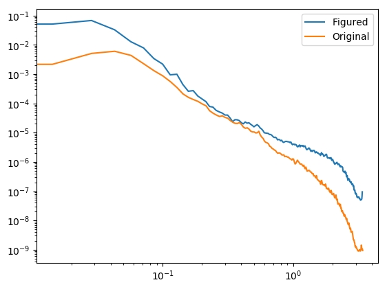
ps = Dl.psd(analysis=True)
WARNING: low limit detected in prange, can cause problems with log color scale.
<Figure size 640x480 with 0 Axes>

ps.plot()
<Axes: title={'center': '2D PSD'}, xlabel='X (um)', ylabel='freq. (um$^{-1}$)'>

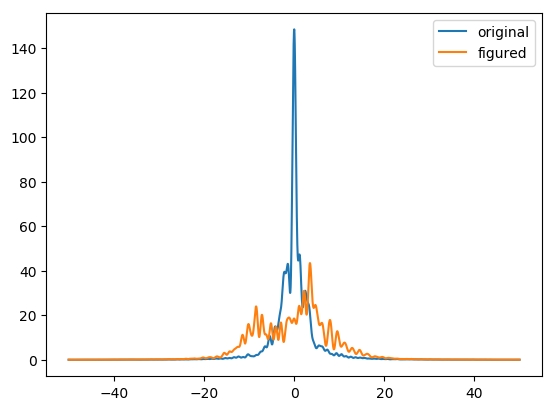
from pyProfile.psd import plot_psd

plot_psd(*ps.avgpsd())
No handles with labels found to put in legend.

Gallery
Applicable cases in my experience:
- Batch extraction of regions, points or profiles from data, calculation of derived quantities and analysis/visualization as series (e.g. time evolution, thermal and environmental effects).
- Best fit of a surface by scaling of another surface (e.g thin films stress), or combination of multiple ones (e.g.: summing deformations);.
- Comparison of two different surface maps with different sampling or registration;
- Combination and stitching of data larger than a single field. (e.g. uniformity obtained by small maps on larger maps).
- Building data pipelines, or in general all cases where a complex analysis on data needs to be repeated multiple times.
- Integration with existing specific code or analysis tools.
Fit of Stress in thin films

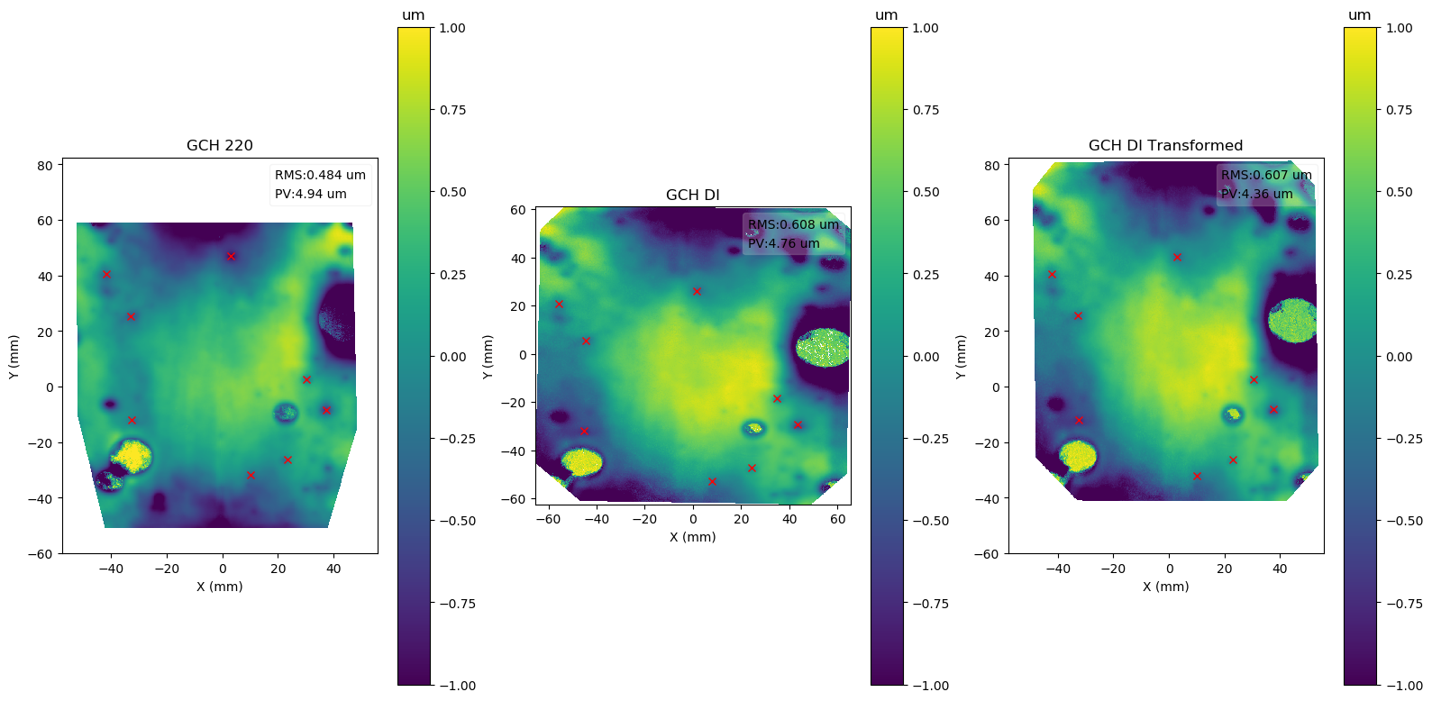
Alignment of Images with different instruments
Slope Analysis
Methods .slope of object data2d_class.Data2D, and functions plot_slope_2D and plot_slope_slice calculate slopes and related statistics.
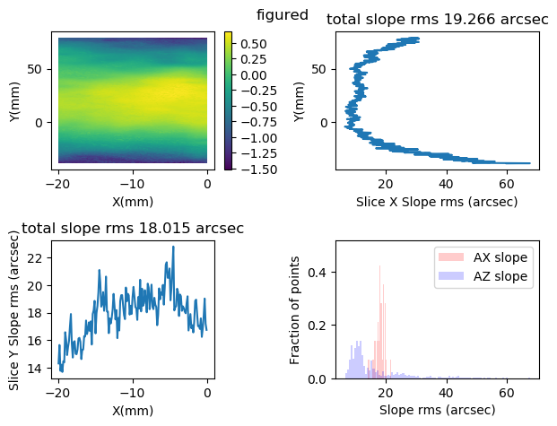
Data2D.slope?
Signature: Data2D.slope(self, *args, **kwargs)
Docstring:
slope_2D(wdata, x, y, scale=(1.0, 1.0, 1.0))
calculate slope maps in x and y.
    return a couple of maps of type slope,x,y data for x and y slopes respectively.
    Set scale to (dx,dy,1000.) for z in micron, x,y in mm. (?does it mean  1,1,1000?)
File:      c:\users\kovor\documents\python\pyxtel\source\pysurf\data2d_class.py
Type:      function
Fit of Model
In this experiment, a part was measured before and after a process.
The two sets of data need to be aligned and subtracted, which can be done
 | |
Results of Machining and Optical Performance Simulation
|  |  |
Extraction of Statistics

Status of the project
- First public appearence, until now a single person project.
- I constantly work on it, as I use it. So this is what dictate my direction, but it can change on user feedback.
- Of course, first thing to make it usable is to have documentation.
- Documentation is available for many functions as docstrings (Python way of automatically generating documentation from comments in code), but is not uniform and not available as external documentation.
- Installation can be (easily) performed manually.
Contacts
Project page (docs):
Source Code: https://github.com/vincenzooo/pyXsurf
My email: vincenzo.cotroneo@inaf.it
Acknowledgements
Thanks to my current Institution (Osservatorio Astronomico di Brera, Merate, IT) and the previous one (Center for Astrophysics | Harvard & Smithsonian, Cambridge, MA, USA).
Thanks to the wonderful Python community.